This is a class summary of AAI5003, 2021 spring semester lectured by Jinyoung Yeo at Yonsei University.
Before we start, assuming that we are all new to NLP, let’s think how to input words into neural networks. If you are familiar with machine learning techniques, we already know that one-hot encoding can replace categorical values into numeric values, which is interpretable for our NN model. However, the problem is that there are too many words we have to input. Even a single sentence like “Last week, I saw Interstellar with a blind date, and it was so fun that I explained about the black hole to her in a cafe for an hour, but now no message from her, but it’s okay because this movie was really amazing.” consists about 40 words, resulting in cardinality issues. In this case, the one-hot represented matrix is so sparse that it requires more memory and computational time but has poor information quality. Thus, the needs for conveying word information, preserving the original context, have emerged.
1. Dimensionality Reduction
There are widely-used dimensionality reduction methods such as PCA (Principal Component Analysis) and LDA (Linear Discriminana Analysis) but we are going to cover AutoEncoder in this post.
AutoEncoder
Actually, AutoEncoder is one unsupervised neural network model with low depth of layers and small number of hidden layers. On the other hand, AutoEncoder functions as a feature extractor, reducing dimensionality of inputs.
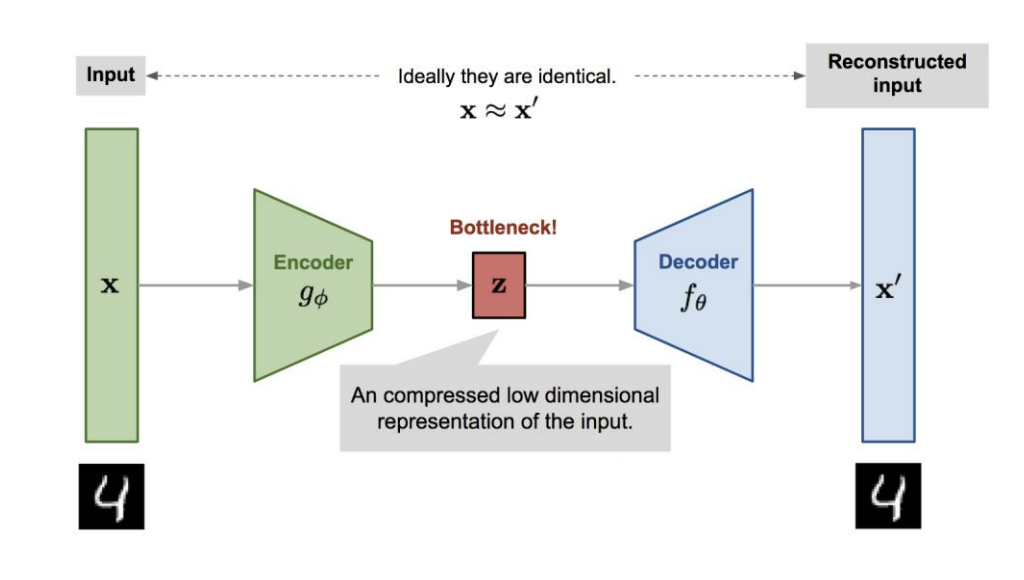
See its simplified structure first:

AutoEncoder consists of two parts: Encoder and Decoder.
- Encoder: Compress input data into smaller dimension (Z)
- Decoder: Decompress/Reconstruct compressed vector (Z) that assembles X most
While encoding, the model automatically learns important features of input data that we call it feature extractor. We can input this compressed input data, Z, into our neural networks. (Forget the decoder here!)
For Torch implementation, read this
2. Word Embedding: Word2Vec
However, previous dimensionality reduction methods such as AutoEncoder is problematic in NLP since it independently covers individual inputs. The meaning of a word heavily depends on neighboring words and context but the original one-hot encoded method cannot capture those characteristics of words.
To solve this, Word2Vec uses neighboring words of our target word.
For example, there are two sentences like
President Moon said yesterday…
President Biden said yesterday…
Considering that Moon and Biden share similar contexts, we can infer that they are similar.
Word2Vec came out from this idea: **Similar contexts share similar meanings! **
There are two ways to implement Word2Vec: CBOW, Skip-gram.
Continuous Bag of Words (CBOW)
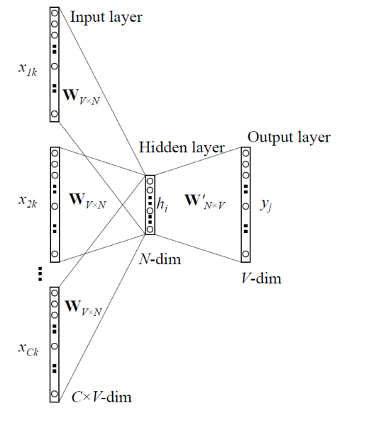
CBOW predicts one single word based on neighboring words. Assume that there is a sentence like
… The White House is expected to announce a target to cut emissions …
Then the input data is The, White, House, is, expected, to, a, target, to, cut, emissions and the output, our target is announce.
INPUT: neighboring C words ($x_{1k}, x_{2k}, … , x_{Ck}$)
OUTPUT: a single word ($y_j$)

Skip-gram
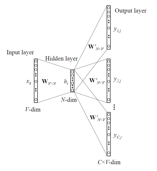
Skip-gram flips the CBOW model structure. It predicts neighboring words by a single word.
From the previous example, in Skip-gram, the input data is announce but the target data is The, White, House, is, expected, to, a, target, to, cut, emissions.
INPUT: a single word ($x_k$)
OUTPUT: sets of neighboring C words ($y_{1j}, y_{2j}, …, y_{Cj}$)

In both ways, the input word is a one-hot vector so $h$ after the hidden layer works as an embedded word vector. For details, look at this simple example.

Since the input data is a one-hot encoded vector, the hidden layer is like a lookup table where each row is an embedded vector for each input word. It also applies to Skip-gram.
CBOW is faster than Skip-gram but Skip-gram works well with even small training datasets.
Reference
- https://lilianweng.github.io/lil-log/2018/08/12/from-autoencoder-to-beta-vae.html
- https://reniew.github.io/21/